
OCR A Physics H556 · Module 3 · Forces and motion
Springs: Hooke’s law, series and parallel, and elastic energy
Why does adding a spring sometimes make a support softer and sometimes make it stiffer? Follow the forces and extensions, then use energy to predict what happens when a spring launches, stops or supports a moving object.
Specification: 3.4.1(a–d); 3.4.2(a–c), (e–f); energy applications from 3.3.1(c–e) and 3.3.2(a–c)
Start with a prediction
Two identical springs support the same total load. One arrangement connects them end to end; another holds them side by side at equal extension. Which arrangement extends further? Would the answer change if you fixed the extension instead of the load?
Check your prediction
For the same total force, the series chain extends further: both springs carry that force and their extensions add. In parallel they share the load. At the same extension the parallel pair instead needs more force. Always state which quantity is fixed.
Before you start: Work and energy · Forces and free-body diagrams.
By the end you should be able to
- Distinguish extension, compression, elastic and plastic deformation.
- Determine a force constant and state the limit of Hooke’s law.
- Derive and apply equivalent stiffness for series, parallel and mixed spring arrangements.
- Calculate component forces, extensions and stored energies in a spring network.
- Use force–extension graph area and distinguish loading work, returned energy and dissipation.
- Apply conservation of energy to spring launches, compression and vertical motion.
- Distinguish a turning point from an equilibrium position.
- Compare typical ductile, brittle and polymeric stress–strain behaviour.
- Plan a loading/unloading investigation and evaluate its measurements.
One spring: force, length and extension
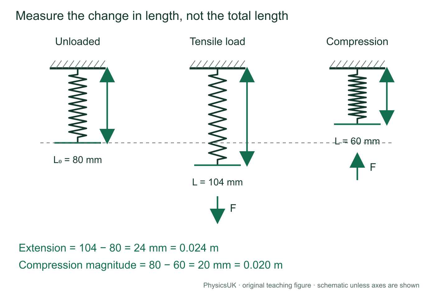
A tensile force stretches an object; a compressive force shortens it. Measure the change from a stated reference length. A spring that is 104 mm long has not necessarily extended by 104 mm.
L0 is the unloaded length and L is the loaded length, both in metres. F is the magnitude of the applied axial force in newtons. The force constant k measures stiffness, in N m−1. A larger k means a larger force is needed for the same extension. For compression, use its positive magnitude unless a signed coordinate is explicitly defined.
Hooke’s law states that extension or compression is directly proportional to the applied force within the proportional range. Doubling the force then doubles the change in length. The spring’s restoring force acts against the deformation: with a signed displacement from natural length, Fspring = −kx.
Scroll across on a narrow screen, or open the figure for a larger view.
Worked example 1: find the stiffness
A spring has unloaded length 80.0 mm. A 3.60 N tensile force increases its length to 104.0 mm within its proportional range. Find k.
- x = 104.0 − 80.0 = 24.0 mm = 0.0240 m.
- k = F/x = 3.60/0.0240 = 150 N m−1.
- Check: 150 × 0.0240 = 3.60 N. Using total length 0.104 m would describe the wrong deformation.
Elastic is not the same as Hookean
An elastic deformation is recovered when the force is removed. A plastic deformation leaves a permanent change. The limit of proportionality ends the straight-line region; the elastic limit marks the onset of permanent deformation. They need not coincide. A rubber strip can recover its shape even with a curved force-extension graph.
Use the following equations for light, linear, reversible springs within their proportional ranges. Unless stated otherwise, connectors are light and friction, air resistance and energy left in spring motion are neglected. Real springs can have preload, slack, hysteresis or permanent deformation.
Springs in series: same force, extensions add
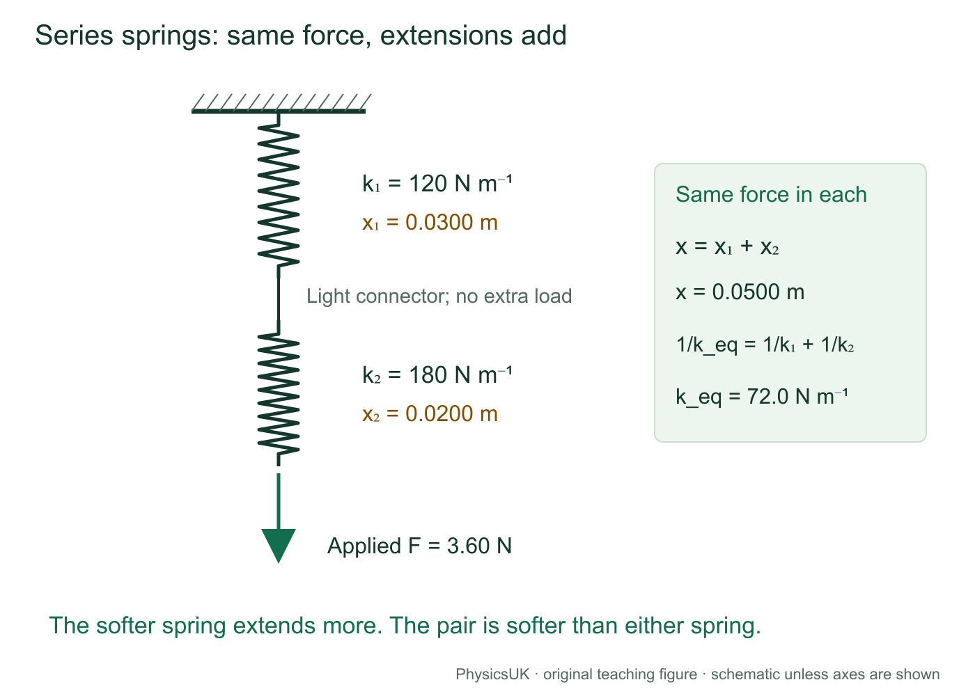
Connect two springs end to end with a light connector and no extra junction load. The connector has negligible weight and is in equilibrium, so the two spring forces on it have equal magnitudes. Each spring carries the same axial force F. Total extension is the sum of the individual extensions.
Force and geometry
x = x1 + x2
x1 = F/k1 and x2 = F/k2.
Equivalent spring
Define F = keqx. Then F/keq = F/k1 + F/k2.
Divide by the common nonzero F.
For n identical springs, keq = k/n. The combination is softer than any individual spring: the same load produces several extensions that add. Unequal springs generally have unequal extensions; the softer one extends more because x = F/k.
Scroll across on a narrow screen, or open the figure for a larger view.
Worked example 2: unequal springs in series
Springs of 120 and 180 N m−1 carry a 3.60 N axial load in series.
- keq = (120 × 180)/(120 + 180) = 72.0 N m−1.
- x1 = 3.60/120 = 0.0300 m; x2 = 3.60/180 = 0.0200 m.
- Total extension = 0.0500 m.
- Check: F/keq = 3.60/72.0 = 0.0500 m.
Do not split the 3.60 N between the springs: the load is transmitted through the chain.
If another mass or external force acts at the junction, the two tensions need not be equal. Draw the junction’s forces before using the simple series rule.
Springs in parallel: same extension, forces add
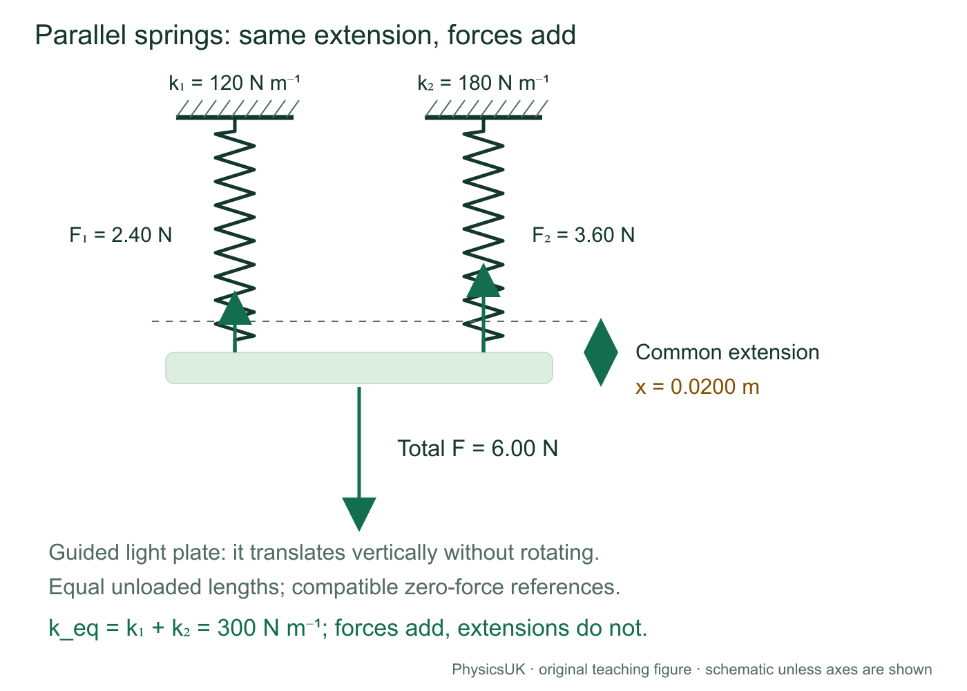
Attach two initially unstrained springs between a fixed support and a light plate that can move vertically but cannot rotate. With equal unloaded lengths, both have the same extension x. Their upward forces add: F = F1 + F2.
For n identical parallel springs, keq = nk. The combination is stiffer because several springs oppose the same movement. For unequal stiffnesses, equal extension does not mean equal force: F1/F2 = k1/k2.
Scroll across on a narrow screen, or open the figure for a larger view.
Worked example 3: share a load between unequal springs
The same 120 and 180 N m−1 springs form this parallel arrangement under a total 6.00 N load.
- keq = 120 + 180 = 300 N m−1.
- Common extension x = 6.00/300 = 0.0200 m.
- F1 = 120 × 0.0200 = 2.40 N; F2 = 180 × 0.0200 = 3.60 N.
- Check: forces sum to 6.00 N. Their 2:3 ratio matches the stiffness ratio.
Springs drawn side by side are not automatically a simple parallel pair. If a bar can tilt, unloaded lengths differ, or a spring is preloaded or slack, establish each extension and the force balance first.
| Feature | Simple series chain | Simple parallel pair |
|---|---|---|
| Shared quantity | Axial force | Extension |
| Quantity that adds | Extensions | Forces |
| Two identical springs, each stiffness k | keq = k/2 | keq = 2k |
| Useful check | Softer than either spring | Stiffer than either spring |
Mixed combinations: reduce a group, then work back
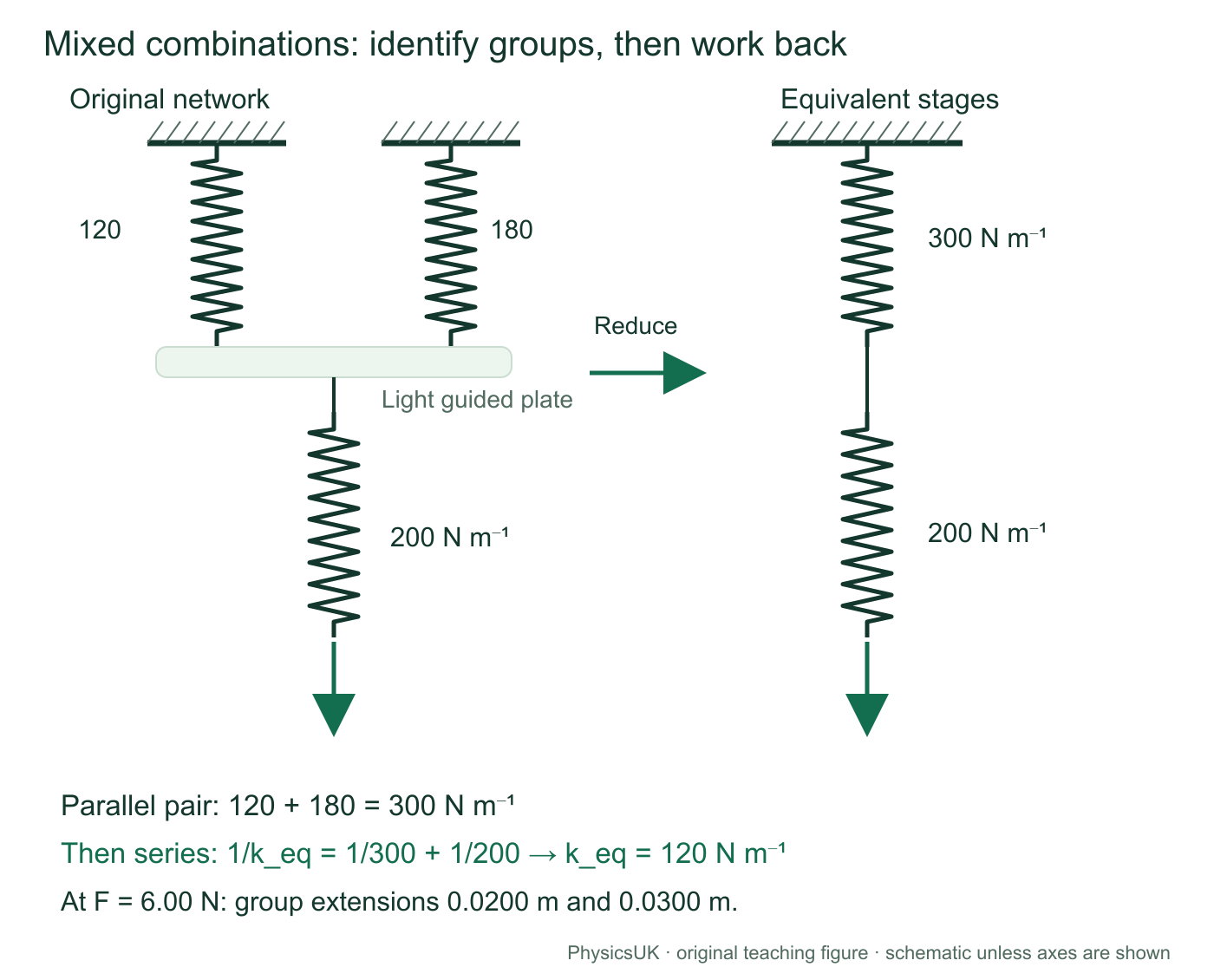
Start with attachment points and permitted motion. Identify a group with the same force or the same extension; replace it by an equivalent spring. Repeat only while those physical conditions hold. A complicated drawing is not a reason to add every k.
Scroll across on a narrow screen, or open the figure for a larger view.
Worked example 4: a parallel pair in a series chain
The diagram’s network carries a 6.00 N axial load. Find total extension, the extension and force of each spring, and total stored energy.
- Parallel group kP = 120 + 180 = 300 N m−1.
- Then keq = (300 × 200)/(300 + 200) = 120 N m−1.
- Total extension = 6.00/120 = 0.0500 m.
- Each series group carries 6.00 N: xP = 6.00/300 = 0.0200 m; x3 = 6.00/200 = 0.0300 m.
- Each parallel spring extends by 0.0200 m; their forces are 2.40 N and 3.60 N. The third spring carries 6.00 N.
- Using the energy equation derived next, individual energies are ½ × 120 × 0.0200² = 0.0240 J, ½ × 180 × 0.0200² = 0.0360 J and ½ × 200 × 0.0300² = 0.0900 J.
Total energy = 0.150 J. Check: ½keqx² = ½ × 120 × 0.0500² = 0.150 J. Components use their own extensions; the equivalent spring uses total extension.
Check a limiting case
If the 200 N m−1 spring became extremely stiff, its extension would become negligible. The network would approach the 300 N m−1 parallel group, not become infinitely stiff: a compliant group remains in the series path.
Work and elastic energy come from graph area
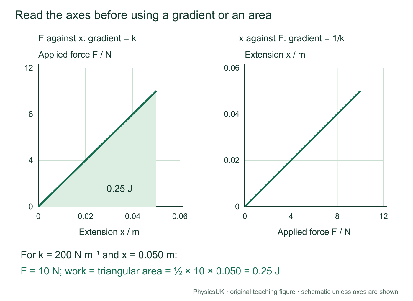
Work done by a changing stretching or compressing force is the area under its force-displacement graph. For linear loading from zero to final force F, the average force is F/2. The area is a triangle, not the rectangle Fx.
These expressions give stored elastic potential energy for a linear, reversible spring, with extension or compression magnitude x measured from its unstrained length. Units are joules because N × m = J. Using Fx would incorrectly apply the final force throughout the change in length.
Scroll across on a narrow screen, or open the figure for a larger view.
At x = 0.0500 m, a 200 N m−1 spring stores ½ × 200 × 0.0500² = 0.250 J. Equivalently, ½ × 10.0 × 0.0500 = 0.250 J. Doubling extension within the proportional range gives four times the energy.
Which quantity stays fixed?
Same extension
E = ½kx²: larger k stores more energy for the same x. Two identical parallel springs store twice the energy of one at that extension.
Same total force
E = F²/(2k): smaller k stores more energy for the same F because it extends further. Two identical series springs store twice the energy of one under that force.
For an ideal network, add Σ½kixi² or use ½keqxtotal² under the same references and constraints. An energy comparison must state what is held fixed.
Curved loading and unloading graphs
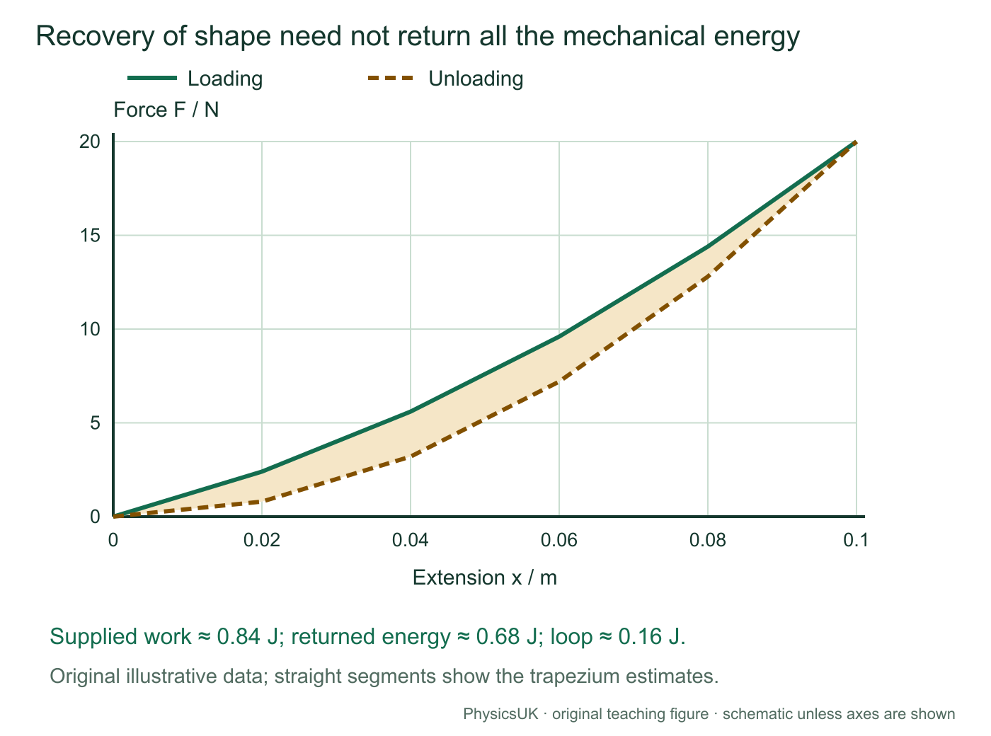
For a curved graph, estimate area with squares or trapezia and the actual axis units. Do not use ½Fx merely because the object recovers its shape. The loading area is work supplied; the unloading area is energy returned mechanically. The area between them is energy not returned mechanically, typically increasing internal energy and transferring energy to the surroundings.
| Extension x / m | 0.00 | 0.02 | 0.04 | 0.06 | 0.08 | 0.10 |
|---|---|---|---|---|---|---|
| Loading force / N | 0 | 2.4 | 5.6 | 9.6 | 14.4 | 20.0 |
| Unloading force / N | 0 | 0.8 | 3.2 | 7.2 | 12.8 | 20.0 |
Scroll across on a narrow screen, or open the figure for a larger view.
Worked graph analysis: estimate both areas
Using 0.02 m-wide trapezia, loading work ≈ 0.02[½(0 + 20) + 2.4 + 5.6 + 9.6 + 14.4] = 0.84 J. Returned energy ≈ 0.02[½(0 + 20) + 0.8 + 3.2 + 7.2 + 12.8] = 0.68 J. Difference ≈ 0.16 J. These are estimates from the supplied intervals, not exact integrals of a known experimental curve.
Energy transfers: define the initial and final states
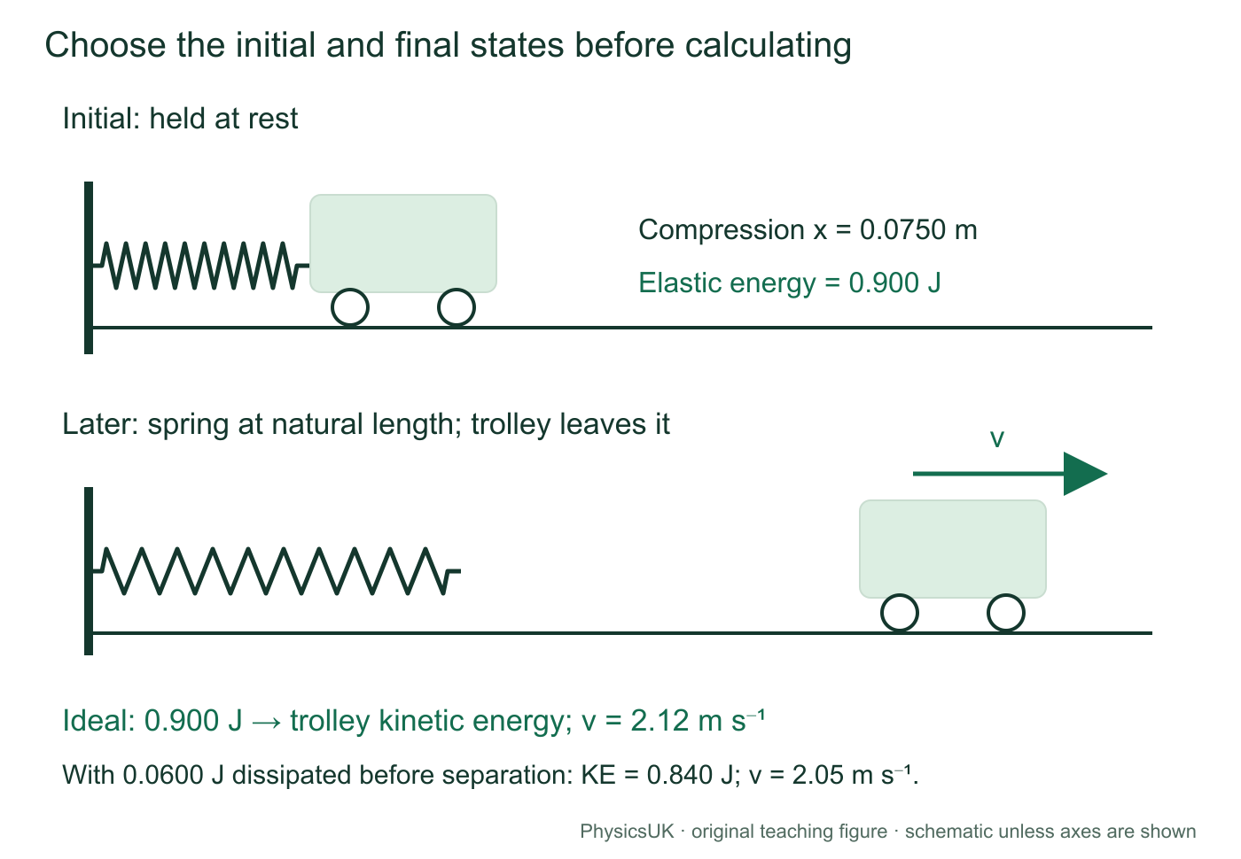
A spring can launch a trolley, stop a moving object or change its height. Choose the system and two states, then account for every relevant energy store. Spring force varies, so constant-acceleration equations do not generally describe the spring-driven stage.
KE = ½mv²; changes in GPE are mgΔh in a uniform gravitational field. Energy dissipated is a positive amount removed from the mechanical energy account; total energy is still conserved. Include externally supplied work if there is extra input. The following examples have none.
Scroll across on a narrow screen, or open the figure for a larger view.
Worked example 5: a spring launches a trolley
A 320 N m−1 spring is compressed by 0.0750 m against a 0.400 kg trolley at rest on a horizontal track. The trolley is not attached to the spring. Find its speed when the spring reaches natural length.
- Initial spring energy = ½ × 320 × 0.0750² = 0.900 J.
- In the ideal model, final spring energy is zero and there is no height change: ½ × 0.400 × v² = 0.900.
- v = √(2 × 0.900/0.400) = 2.12 m s−1.
- If 0.0600 J is dissipated before separation, final KE = 0.900 − 0.0600 = 0.840 J, giving 2.05 m s−1 at natural length.
Check: allowing losses reduces speed. With dissipation, the greatest speed may occur before separation; this energy account gives speed at separation, not automatically maximum speed.
Reverse the transfer: a moving object compresses a spring
For an incoming object on a level frictionless track, maximum compression is a turning point: v = 0 instantaneously. With an initially unstrained spring, ½mu² = ½kx², so x = u√(m/k), where u is the incoming speed. The object is not in equilibrium there: the spring accelerates it back. Question 8 applies this.
Include gravity when height changes
If spring release takes a trolley up an incline, initial spring energy supplies final KE, the gain mgΔh and any dissipation. Use the height change between your chosen states, not necessarily the distance travelled. Do not equate all spring energy to KE while the object gains height.
Scroll across on a narrow screen, or open the figure for a larger view.
Worked example 6: a mass falls while stretching a spring
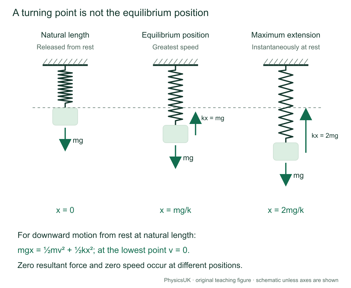
A 0.200 kg mass is attached to a light vertical spring, k = 80.0 N m−1. It is released from rest with the spring initially at natural length. Neglect damping; use g = 9.81 m s−2. Find equilibrium extension and maximum extension on the first fall.
- Equilibrium is a force condition. kxeq = mg, so xeq = (0.200 × 9.81)/80.0 = 0.0245 m.
- The lower turning point is an energy condition. Downward extension x lowers the mass by x: lost GPE becomes spring energy and KE, so mgx = ½mv² + ½kx².
- At maximum extension v = 0, so mgx = ½kx². Apart from the initial x = 0 solution, xmax = 2mg/k = 0.0491 m.
- Check: spring energy = ½ × 80.0 × 0.04905² = 0.0962 J, matching the lost GPE mgx.
The mass is fastest at equilibrium, where resultant force changes from downwards to upwards. At the lowest point, spring force is 2mg and resultant force is mg upwards, even though speed is momentarily zero. These results require release from rest at natural length; they are not rules for every vertical spring motion.
PAG 2: measure force-extension characteristics
Measure the response rather than assuming every spring, rubber band or polythene strip has one constant k. Use a load range suitable for the specimen and apparatus.
- Clamp the upper end securely. Place a fixed ruler beside a clear pointer and stable reference mark. Record unloaded length L0; state whether a hanger or preload is already present.
- Add known masses in steps. For a stationary suspended load, calculate F = mg, including the hanger when it contributes to that load. Mass in kilograms is not force in newtons.
- Wait for motion to settle; read at eye level to reduce parallax. Calculate L − L0. Use enough points to reveal curvature, with smaller steps near a change in behaviour.
- Unload in steps and record lengths again. Label both curves and check for genuine residual extension after removing the load.
- Repeat to assess scatter. Keep temperature and loading time/rate consistent, particularly for polymers that creep. Secure the stand, use suitable eye protection and a tray beneath masses, and stay within safe load limits.
Choose and analyse the graph
For linear F against x, k = ΔF/Δx. Use two well-separated points on the fitted line, not necessarily measured points. With x against F, gradient = 1/k. Convert mm or cm to metres before reporting k in N m−1.
With extension against added mass M, a linear model can be x = (g/k)M + c. Gradient = g/k, so k = g/gradient. An intercept c can reflect a hanger or preload when the horizontal axis contains only added mass. Interpret the stated reference: a nonzero intercept on that graph is not by itself proof of non-Hookean behaviour.
Extension is a difference between two lengths. For a conservative maximum absolute uncertainty, add their absolute reading uncertainties. Two readings of ±0.5 mm give up to ±1.0 mm in extension by that method. Repeats assess random scatter but do not remove a shifted zero or slipping clamp.
Worked practical check: an uncertain gradient
An extension-on-force best-fit gradient is 0.0100 m N−1; a worst acceptable gradient is 0.0108 m N−1. The corresponding k values are 100 and 92.6 N m−1. Comparing k gives a 7.4% deviation. The gradient changes by 8.0%; the fractional-uncertainty approximation for a reciprocal gives about 8%, close to but not exactly the finite reciprocal change.
A worst acceptable line must be consistent with all stated error bars, not arbitrarily steep or shallow. If both extremes are available, compare the relevant limiting k values and state the uncertainty convention.
A constant preload can establish a repeatable reference. Label additional force and additional extension if using that state as zero. Check ruler alignment, support movement and pointer attachment before interpreting apparent permanent extension.
Compare material behaviour without confusing the properties
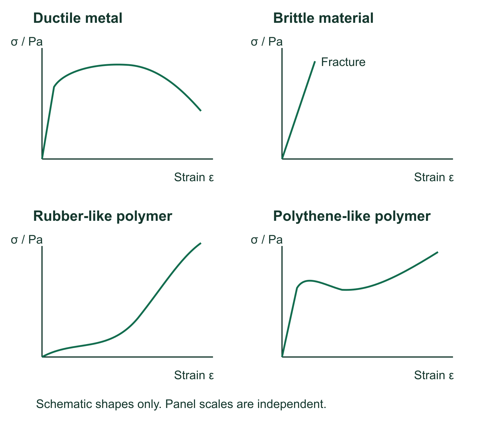
Force constant describes a specimen. Stress σ = F/A0 uses original cross-sectional area and is measured in Pa. Strain ε = ΔL/L0 is dimensionless. Young modulus is the initial linear stress-strain gradient. Ultimate tensile strength is maximum tensile force divided by original area.
Scroll across on a narrow screen, or open the figure for a larger view.
| Typical behaviour | Graph and recovery | Interpretation |
|---|---|---|
| Ductile metal | Elastic region, then substantial plastic strain before fracture; engineering stress can fall after its maximum during necking. | Considerable permanent deformation before fracture; not every metal has a sharply defined yield point. |
| Brittle material, such as glass | Little plastic strain before fracture; often approximately linear over its small strain range. | Brittle does not necessarily mean low strength or low stiffness. |
| Rubber-like polymer | Large recoverable strains, a curved loading relation and possibly an unloading loop. | Elastic need not mean Hookean or complete mechanical-energy recovery. |
| Polythene-like polymer | May yield and retain large permanent extension; response can depend on time. | A material family does not have one universal graph. |
For a uniform straight wire in the linear range, k = EA0/L0. A thicker or shorter wire can have larger k without changing the material’s Young modulus E. High Young modulus does not automatically mean high breaking stress or large breaking strain. The Young modulus investigation covers the detailed wire apparatus and uncertainty method.
Independent exam practice
These are original PhysicsUK questions and marking guidance, not official OCR questions or approved mark schemes. Use g = 9.81 m s−2 where needed. Unless stated otherwise, assume light linear reversible springs, light connectors, negligible friction and drag. Show working, units and the physical condition used.
Questions 1–10: 46 marks. Three material checks add 9 marks. Try each question before opening its answer. For Question 2, draw your graph on paper or with graphing software.
1. Measure a stiffness (3 marks)
A spring extends by 28.0 mm under an applied force of 4.20 N. Calculate its force constant. State the condition needed to use Hooke’s law over this interval.
Show solution and mark scheme
- x = 28.0 × 10−3 = 0.0280 m. [1]
- k = F/x = 4.20/0.0280 = 150 N m−1, including the unit. [1]
- Force and extension are directly proportional over the interval, within the proportional range. “It is elastic” alone is insufficient. [1]
2. Graphs and a practical method (6 marks)
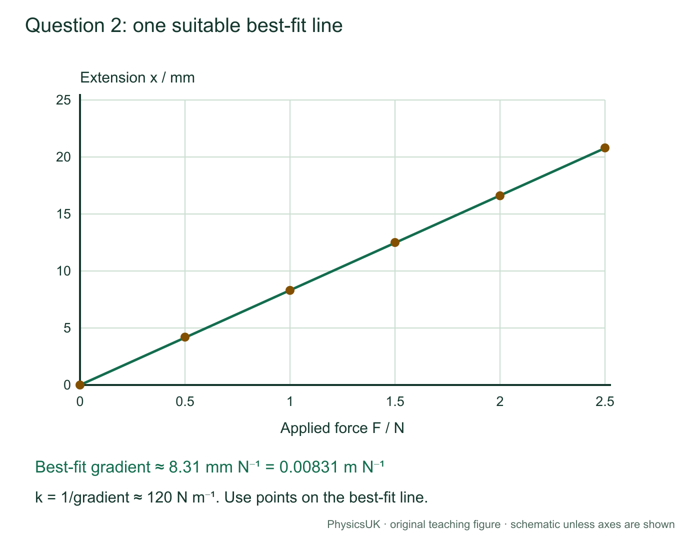
These original illustrative measurements use the whole suspended load as force and the same unloaded reference for extension.
| Applied force F / N | 0.00 | 0.50 | 1.00 | 1.50 | 2.00 | 2.50 |
|---|---|---|---|---|---|---|
| Extension x / mm | 0.0 | 4.2 | 8.3 | 12.5 | 16.6 | 20.8 |
(a) Plot extension on the vertical axis against force on the horizontal axis, with a straight best-fit line. (2 marks)
(b) Use a large gradient triangle to estimate k in N m−1. (2 marks)
(c) Explain how masses provide the force, and give one specific improvement to length readings. (2 marks)
Show solution and mark scheme
- Axes labelled x / mm and F / N (or a consistently converted metre axis), suitable linear scales and correct points; allow half a small square. [1]
- A sensible straight best-fit line with scatter distributed on either side, not joined successive points. [1]
- A large triangle on the line gives about 8.3 mm N−1 = 0.0083 m N−1, with the conversion shown. [1]
- k = 1/gradient ≈ 120 N m−1. Accept 118–122 N m−1 with suitable graphical working; allow follow-through from a reasonable gradient. [1]
- F = mg for the stationary total suspended mass, including the hanger where relevant. [1]
- One explained improvement: a clear pointer close to the ruler and eye-level readings reduce parallax; a suitably finer scale improves resolution; or repeated settled readings assess random scatter. “Be more accurate” alone is insufficient. [1]
Scroll across on a narrow screen, or open the figure for a larger view.
3. Unequal springs in series (4 marks)
Springs of 90.0 and 180 N m−1 are connected end to end with a light connector and no extra junction load. A steady 2.70 N axial force stretches the chain. Find equivalent stiffness, each extension and total extension.
Show solution and mark scheme
- 1/keq = 1/90.0 + 1/180, so keq = 60.0 N m−1. [1]
- The 90.0 N m−1 spring carries 2.70 N: x1 = 2.70/90.0 = 0.0300 m. [1]
- x2 = 2.70/180 = 0.0150 m. [1]
- Total = 0.0450 m, also given by 2.70/60.0. [1]
The softer spring extends twice as much. Allow consistent follow-through for the total after an isolated component error.
4. A parallel pair shares a load (4 marks)
Initially unstrained springs with equal unloaded lengths and force constants 140 and 210 N m−1 connect a fixed support to a light plate. It translates vertically without rotating; its guides exert no vertical force. Apply a total downward load of 7.00 N. Find the displacement and each spring’s load. Explain why the loads are unequal.
Show solution and mark scheme
- keq = 350 N m−1; x = 7.00/350 = 0.0200 m. [1]
- F1 = 140 × 0.0200 = 2.80 N. [1]
- F2 = 210 × 0.0200 = 4.20 N; together 7.00 N. [1]
- Equal extensions and F = kx give greater force in the stiffer spring. [1]
5. A mixed network and its energy (6 marks)
Use the mixed-network teaching figure’s topology, but replace its parallel springs by 100 and 150 N m−1 springs and its series spring by a 250 N m−1 spring. The parallel pair has equal unloaded lengths and is initially unstrained. Its light plate cannot rotate; guides provide no vertical force. A 5.00 N axial load acts through the network.
Find equivalent stiffness, total and group extensions, and the force in each parallel branch. Calculate total stored energy by adding component energies and using the equivalent spring.
Show solution and mark scheme
- Parallel group kP = 100 + 150 = 250 N m−1. [1]
- Series combination: keq = 250 × 250/(250 + 250) = 125 N m−1. [1]
- Total extension = 5.00/125 = 0.0400 m; each series group extends by 5.00/250 = 0.0200 m. [1]
- Parallel forces = 100 × 0.0200 = 2.00 N and 150 × 0.0200 = 3.00 N. [1]
- Individual energies = 0.0200 + 0.0300 + 0.0500 = 0.100 J, using each spring’s own extension in ½kx². [1]
- Equivalent check: ½ × 125 × 0.0400² = 0.100 J, agreeing with the sum. [1]
Allow consistent follow-through after a stiffness error if component and equivalent methods use the appropriate extensions.
6. Explain an energy graph (4 marks)
A spring’s linear force-extension graph passes through the origin and x = 0.0400 m, F = 12.0 N. Explain how the graph gives stored energy and calculate it. Predict the energy change if extension doubles within the proportional, reversible range.
Show solution and mark scheme
- Work done, here stored elastic energy, is area under the force-extension graph. [1]
- The region is triangular, so E = ½Fx, not Fx. [1]
- E = ½ × 12.0 × 0.0400 = 0.240 J. Using k = 300 N m−1 is also valid. [1]
- E ∝ x² for fixed k: doubling x gives four times the energy, 0.960 J. [1]
7. Launch a trolley, with and without losses (4 marks)
A 250 N m−1 spring is compressed by 0.0800 m against a 0.500 kg trolley at rest on a level track. The trolley is not attached to the spring. Find initial elastic energy and speed at natural length in the ideal model. Then find its KE and speed there if 20.0% of initial spring energy is dissipated before separation.
Show solution and mark scheme
- E = ½ × 250 × 0.0800² = 0.800 J. [1]
- Ideal ½mv² = 0.800 gives v = √(2 × 0.800/0.500) = 1.79 m s−1. [1]
- With losses, KE = 0.800 × 0.800 = 0.640 J. [1]
- v = √(2 × 0.640/0.500) = 1.60 m s−1. [1]
Allow follow-through from energy. Losing 20% of energy does not mean losing 20% of speed because KE depends on v².
8. Stop a moving trolley (4 marks)
A 0.300 kg trolley at 1.80 m s−1 meets an initially unstrained 240 N m−1 spring on a level frictionless track. Find maximum compression and explain why zero speed there does not mean zero resultant force.
Show solution and mark scheme
- At maximum compression, initial KE becomes spring energy: ½mu² = ½kx². [1]
- Initial KE = ½ × 0.300 × 1.80² = 0.486 J. [1]
- x = √(2 × 0.486/240) = 0.0636 m. [1]
- It is a turning point: v = 0 momentarily but the compressed spring exerts a restoring force, accelerating the trolley back. [1]
9. Equilibrium or a turning point? (6 marks)
A 0.180 kg mass is attached to a light vertical spring, k = 90.0 N m−1. Release it from rest at natural length. Find equilibrium extension and maximum extension on its first fall. Explain the motion and forces at equilibrium and the lowest point.
Show solution and mark scheme
- At equilibrium, kxeq = mg. [1]
- xeq = (0.180 × 9.81)/90.0 = 0.0196 m. [1]
- At the lower turning point KE = 0, so lost GPE becomes spring energy: mgx = ½kx². [1]
- Nonzero solution: xmax = 2mg/k = 0.0392 m. [1]
- At the lowest point speed is zero but kx = 2mg, leaving resultant force mg upwards: not equilibrium. [1]
- At equilibrium resultant force is zero and changes direction as the mass passes through, so speed is greatest there. [1]
Do not use kx = mg at maximum extension. The factor of two is specific to this release and ideal model.
10. An unfamiliar loading cycle (5 marks)
A specimen’s loading graph is curved. It receives 1.40 J on loading and returns 1.05 J mechanically on unloading, recovering its original length. Decide whether it is elastic and whether Hooke’s law applies over the whole range. Calculate the energy not returned and percentage returned, and explain where the missing mechanical energy can go.
Show solution and mark scheme
- Elastic in the stated sense: it recovers its original length. [1]
- A curved force-extension relation is not direct proportionality, so Hooke’s law does not describe the whole range. [1]
- Not returned: 1.40 − 1.05 = 0.350 J. [1]
- Percentage returned = 100 × 1.05/1.40 = 75.0%. [1]
- Mechanical energy can increase the specimen’s internal energy and transfer to its surroundings, for example by heating. It is not destroyed. [1]
Material checks: 9 further marks
11. Identify the behaviour (4 marks)
Specimen A fractures with little plastic strain. B undergoes extensive plastic strain before fracture. C shows large recoverable strain with a curved force-extension graph. Classify A and B, describe C, and explain why this alone cannot rank their Young moduli.
Show solution and mark scheme
- A is brittle. [1]
- B is ductile. [1]
- C is elastic but need not be Hookean; rubber-like behaviour is possible. [1]
- Young modulus requires the initial stress-strain gradient with quantitative axes; these qualitative descriptions are insufficient. [1]
12. Ultimate tensile strength (3 marks)
A sample has original cross-sectional area 0.800 mm² and maximum tensile force 480 N. Find ultimate tensile strength and distinguish it from Young modulus.
Show solution and mark scheme
- A0 = 0.800 × 10⁻⁶ m². [1]
- UTS = Fmax/A0 = 6.00 × 10⁸ Pa = 600 MPa. [1]
- Young modulus is the initial linear stress-strain gradient, not maximum stress. [1]
13. Check the zero-load reference (2 marks)
After unloading, a strip remains 4 mm longer than its original unloaded length. What does this show, and what reference-reading check should you make first?
Show solution and mark scheme
- A genuine residual extension shows plastic deformation. [1]
- Check the same zero-load reference and that clamps, support or pointer have not moved; a changed reference can mimic residual extension. [1]
Before you move on
- Length is not extension: x = L − L0; convert to metres for k in N m−1.
- Read axes: F-on-x gradient = k; x-on-F gradient = 1/k; x-on-mass gradient = g/k for the stated model.
- Series: same force, extensions add. Parallel: same extension, forces add, when the constraints establish those conditions.
- Energy: area under F against x. For linear reversible springs, E = ½Fx = ½kx² = F²/(2k).
- State what stays fixed: energy comparisons differ for fixed force and fixed extension.
- Choose states: include kinetic, elastic and gravitational energy, plus specified dissipation or external work.
- A turning point is not equilibrium: zero speed does not mean zero resultant force.
- Elastic need not be Hookean: shape recovery, proportionality and full mechanical-energy recovery are separate tests.
Spring combinations apply force balance, geometry and Hooke’s law. The specification does not name every combination formula as a separate recall outcome. Periods and phase belong to the Module 5 SHM note.
Specification and next steps
OCR A Physics H556, specification version 3.0 (March 2026), Module 3. This note covers shared AS/A-level core content.
| Official reference | Teaching | Practice |
|---|---|---|
| 3.4.1(a–c) | Deformation, Hooke’s law and force constant | Try Q1 |
| 3.4.1(d)(i–ii) | Force graphs and practical methods | Try Q2 |
| Applications of 3.4.1(c) | Series springs: same force, added extensions | Try Q3 |
| Applications of 3.4.1(c) | Parallel springs: same extension, added forces | Try Q4 |
| Applications of 3.4.1(c), 3.4.2(b) | Mixed arrangements and component energy checks | Try Q5 |
| 3.4.2(a–b) | Work, stored energy and loading/unloading areas | Try Q6 |
| 3.3.1(c–e), 3.3.2(a–c); 3.4.2(b) | Spring energy transfers and vertical force/energy conditions | Try Q9 |
| 3.4.2(c), (e–f) | Stress/strain/UTS and material comparisons | Try Q11 |
Official OCR A Physics specification